What is attention? The mechanism behind every modern LLM

By Priya Patel, Insightful AI Desk

The most consequential AI architecture of the 2020s — the transformer — is built on one idea. That idea has a name everyone has heard but few can explain clearly: attention.

This post explains exactly what attention is, why it works, and what it does to the rest of the model. We walk through the math one term at a time, build the intuition for why scaled dot-product attention is the version everyone uses, and then trace how the same mechanism scales up to multi-head attention, cross-attention, and the variants that show up in 2026 frontier models.

🎯 Companion lab: to experiment with the math live, open Attention, Visualized — type a sentence, click any word, and see the attention weights compute in real time.

1. The problem attention solves

Before attention, the dominant way to process a sentence was the recurrent neural network (RNN), and later its more capable cousins the LSTM and GRU. These models read a sentence one word at a time, left to right, maintaining a "hidden state" — a fixed-size vector that supposedly captured everything important about the words seen so far.

The architecture was elegant but had three problems that compounded as sentences grew longer.

Forgetting. A fixed-size hidden state had to compress 5 words, then 50, then 500. By the time the model reached word 500, the information from word 1 had passed through 499 update steps and was essentially lost, no matter how careful the gating mechanism. The "long-term dependency" problem in RNNs was not a bug — it was the architecture telling the truth about its capacity.

Sequential compute. Each step depended on the previous one, so the model couldn't process tokens in parallel. Training a transformer with 1,000-token sequences on the same hardware would later turn out to be roughly 100× faster than training an RNN on the same data — entirely because of this single architectural difference.

Opacity. When an RNN got an answer right, you couldn't easily tell what part of the input it had relied on. The hidden state was a soup. Debugging meant guessing.

Bahdanau et al. introduced attention in 2014 for machine translation, originally as an addition to a recurrent encoder-decoder model. Their motivation was specifically the long-sentence forgetting problem: rather than compressing the entire source sentence into a single hidden vector before decoding, let the decoder look back at every source word, each step, with different weights.

The intermediate variants — Bahdanau-style additive attention, Luong-style multiplicative attention, content-based versus location-based — are mostly of historical interest now. The architecture that subsumed all of them, and is the only one you need to understand, is the scaled dot-product self-attention from Vaswani et al. 2017's Attention Is All You Need.

That paper didn't add attention to a recurrent model. It removed the recurrence entirely. Everything is attention. The result, the transformer, became the foundation of GPT, BERT, T5, Llama, Claude, Gemini — every frontier large language model in 2026 is, at its core, a stack of attention layers.

2. What attention actually does

Here is the entire idea in one sentence:

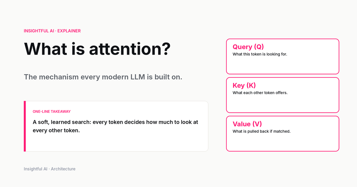
For every token in the input, decide how much to look at every other token — including itself — before deciding what that token means in context.

Read it twice. Everything from here is a way to write that down precisely.

Take the sentence: The cat sat on the mat because it was tired.

The word "it" is ambiguous. It could refer to "cat" or to "mat". A human knows it's the cat because mats don't get tired. For a model to know this, the representation of "it" needs to absorb information from "cat" — not from "mat", and not equally from every other word. The model must attend more to "cat" than to the other tokens.

Attention is the mechanism that does exactly that. For the token "it", attention produces a weighted sum of the surrounding tokens, with the weights deciding how much each source token contributes. If "it" attends 70% to "cat" and 5% each to the other tokens, then the new representation of "it" is 70% "cat-flavored" and ready to be processed by the next layer of the network with that disambiguation already baked in.

The genius is that the model learns these weights. The pattern "pronouns attend to their antecedents" is not coded by humans. It emerges from training on enough text.

▶ Open the lab — try the cat-mat example yourself

3. The search analogy: Q, K, V

The cleanest way to understand attention is to think of it as a soft, learned search.

Imagine a database with 10 records, each with a key (the searchable index) and a value (the actual content). When you query the database, you provide a query, the database compares your query to every key, finds the matches, and returns the corresponding values.

Attention is the soft, continuous, learned version of this:

• Query (Q) — what the current token is looking for
• Key (K) — what each source token offers as its "index"
• Value (V) — what each source token returns if matched

For "it" in our cat sentence, the query might encode "I'm a singular animate pronoun looking for a noun referent." The keys of "cat" and "mat" both encode noun-ness, but "cat" probably has a stronger animate-noun signal. So the query-key similarity for "it"→"cat" is higher than for "it"→"mat", and "it" pulls in more of "cat"'s value than "mat"'s.

The crucial structural fact: Q, K, and V are not three different things that exist in the input. They are three learned linear projections of the same input. The model multiplies the input embeddings by three different weight matrices — $W_Q$, $W_K$, $W_V$ — to produce three views of the same tokens. The model learns through training what to put in each view.

In math, for an input matrix $X$ of shape (sequence length × embedding dim):

$$Q = X W_Q, \quad K = X W_K, \quad V = X W_V$$

Each of $W_Q$, $W_K$, $W_V$ is a learnable parameter matrix. Training adjusts them so that the resulting Q-K similarities produce useful attention patterns — pronouns attending to nouns, verbs attending to subjects, modifiers attending to head nouns.

4. The formula, walked through

Here is the equation everyone writes when they explain attention. It looks intimidating. It isn't.

$$\text{Attention}(Q, K, V) = \text{softmax}\!\left(\frac{QK^T}{\sqrt{d_k}}\right) V$$

Read it left to right, one operation at a time.

$QK^T$. Multiply the query matrix by the transpose of the key matrix. The result is an $N \times N$ matrix where $N$ is the number of tokens. The $(i, j)$ entry is the dot product of the $i$-th query and the $j$-th key — a single number measuring how compatible the $i$-th token's question is with the $j$-th token's offering.

$/\sqrt{d_k}$. Divide every entry by the square root of the key dimension. This is the scaled in "scaled dot-product attention." Without it, when the key dimension is large (in modern LLMs, often 64 or 128 per head), the raw dot products become large and the next step — softmax — saturates into approximately a one-hot vector. The gradient through that softmax then becomes nearly zero, and training stalls. Dividing by $\sqrt{d_k}$ keeps the variance of the dot products roughly constant in $d_k$ and preserves usable gradients.

$\text{softmax}(\cdot)$. Apply softmax row-wise. Each row of the resulting $N \times N$ matrix is now a probability distribution that sums to 1. Row $i$ tells you how much token $i$ attends to each of the $N$ tokens (including itself). High values mean strong attention; near-zero values mean ignore.

$\times V$. Multiply the resulting attention matrix by the value matrix. Each row $i$ of the output is a weighted sum of the value vectors, weighted by the attention probabilities for token $i$. The output of attention is, for every token, a context-aware update derived from the rest of the sequence.

That's all of attention. Four operations: dot product, scale, normalize, weighted sum.

The lab visualization shows exactly this: the heatmap is the softmax-normalized attention matrix. Clicking a token highlights one row of that matrix. The arc visualization is the same matrix, drawn as curves whose thickness encodes weight.

5. Why scaled dot product, specifically

In 2017, there were several attention variants already in circulation. Vaswani et al. chose scaled dot product over additive attention (Bahdanau-style) for one specific reason: speed. The dot product is a single matrix multiplication, highly optimized on GPUs. Additive attention requires a small feed-forward network for every pair of tokens, which doesn't parallelize as well.

The scaling factor $\sqrt{d_k}$ deserves a moment. Suppose Q and K have entries drawn approximately i.i.d. from a distribution with variance 1. Then for two random vectors of dimension $d_k$, the variance of their dot product is approximately $d_k$ (the variance of a sum of $d_k$ independent products is the sum of the variances, each 1). Without scaling, doubling $d_k$ doubles the variance of the pre-softmax scores, which sharpens the softmax exponentially. Sharper softmax means smaller gradients, which means training stalls.

Dividing by $\sqrt{d_k}$ restores variance to roughly 1 regardless of dimension. The choice of $\sqrt{d_k}$ (rather than $d_k$ itself) is the right one because it's the standard deviation, not the variance, that controls the temperature of the softmax.

This is the kind of detail that looks like a hack until you realize it's load-bearing. Without the $\sqrt{d_k}$, deeper transformers would not train. With it, they do.

In the lab, the temperature slider lets you experiment with this directly: higher temperatures spread attention across tokens (like under-scaled scores); lower temperatures focus it on the single most similar token (like a saturated softmax).

6. Multi-head attention

A single attention head learns one kind of pattern. Multi-head attention does several patterns in parallel.

The mechanism is simple. Rather than computing one attention with the full embedding dimension $d_{\text{model}}$, the model splits the embedding into $h$ heads, each of dimension $d_k = d_{\text{model}} / h$. Each head has its own $W_Q$, $W_K$, $W_V$ matrices. The attention computation runs $h$ times in parallel, producing $h$ different attention patterns. The outputs are concatenated and projected back to dimension $d_{\text{model}}$:

$$\text{MultiHead}(Q, K, V) = \text{Concat}(\text{head}_1, \ldots, \text{head}_h) \, W_O$$

$$\text{where head}_i = \text{Attention}(Q W_{Q,i}, K W_{K,i}, V W_{V,i})$$

What do different heads learn? Empirically, in a trained transformer, you can sometimes inspect what each head focuses on. One head might consistently attend to the previous token (capturing local context). Another might attend to syntactic dependencies — verbs attending to their subjects, modifiers to their heads. Another might attend to rare words. The interpretation is fuzzy and contested in the research literature, but the empirical finding is clear: a 12-head attention layer learns 12 noticeably different patterns, each contributing something.

In 2026 frontier models, multi-head attention typically uses between 8 and 128 heads. GPT-4-class models use 96+; smaller open-weight models like Llama 3 use 32. The optimal number depends on the model size and is a hyperparameter chosen during training.

In the lab, try the four head buttons. Each head shows a different attention pattern from random projections (real models train these), so you can see how the same sentence produces different attention weights under different heads.

7. Self-attention vs cross-attention

Everything described so far is self-attention — the queries, keys, and values all come from the same sequence. A token in the input attends to other tokens in the same input.

There's also cross-attention, used in encoder-decoder architectures like the original transformer for translation, T5, and the vision models in CLIP and Flamingo. In cross-attention:

• Queries come from one sequence (e.g., the decoder's tokens so far in translation)
• Keys and values come from another sequence (e.g., the encoder's output for the source sentence)

The math is identical. Only the source of the three projections differs.

GPT-class decoder-only models (everything in the "GPT family", including Claude and Gemini) use only self-attention — they're a single decoder stack with no encoder to cross-attend to. The bidirectional nature of the original transformer's encoder, where every token sees every other, is also self-attention; it's the encoder that doesn't apply a causal mask.

A causal mask is a third common variant. In a decoder generating text left-to-right, token $i$ must not attend to tokens with index $> i$ — otherwise the model could "cheat" by looking at future tokens during training. The mask is a triangular matrix of $-\infty$ values added to the pre-softmax scores, ensuring that softmax assigns zero weight to future tokens. The forward pass is otherwise unchanged.

8. Positional encoding: attention doesn't see order

Here's a fact that surprises people the first time they meet it: attention is permutation-equivariant. If you shuffle the tokens in the input, the attention output shuffles correspondingly, but the pattern of what attends to what is unchanged. Attention has no built-in notion of word order.

This is obviously a problem for language. The cat chased the dog and The dog chased the cat mean very different things, but attention without positional information would compute identical attention weights for both (modulo the labels).

Transformers solve this with positional encoding — extra vectors added to (or combined with) the token embeddings before attention runs, so each token carries information about its position in the sequence.

The original transformer used fixed sinusoidal encodings:

$$\text{PE}_{(\text{pos}, 2i)} = \sin\!\left(\frac{\text{pos}}{10000^{2i/d_{\text{model}}}}\right)$$

$$\text{PE}_{(\text{pos}, 2i+1)} = \cos\!\left(\frac{\text{pos}}{10000^{2i/d_{\text{model}}}}\right)$$

The clever property: differences between positional encodings at different distances are themselves consistent vectors, so the model can learn to extract relative position from the encoding.

Modern models use newer variants. Rotary position embeddings (RoPE), introduced in 2021 by Su et al. and now used in Llama, Gemma, Qwen, and most open-weight LLMs, encode position by rotating the Q and K vectors in 2D pairs by an angle proportional to position. ALiBi (Press et al., 2021) adds a position-dependent linear bias directly to the attention scores instead of modifying embeddings.

The reason there are several variants matters for one practical question: what happens when you try to use a model on sequences longer than it was trained on? Sinusoidal encodings extrapolate poorly; RoPE extrapolates somewhat better; ALiBi was designed specifically for length extrapolation. This is why long-context models — Gemini's 2M context, Claude's 200K, the open-weight community's work on 1M-context Llama variants — pay close attention to positional encoding choice.

9. What attention is not

Two common misconceptions worth correcting.

Attention is not "the model paying attention" in any cognitive sense. It's a weighted sum. The metaphor is useful for intuition but treating it as actual mental attention is misleading. The model doesn't decide what's important the way a person does; it computes dot products, normalizes them, and uses them as weights. Nothing more.

Attention weights are not an explanation. A common idea is that you can inspect attention weights to understand model decisions. Jain and Wallace's 2019 paper Attention is not Explanation argued, with extensive experiments, that attention weights often don't correlate with what actually influences the model's output. You can adversarially permute attention weights and still get the same predictions in many cases. Attention weights are part of the computation, but they are not a faithful explanation of what the model is doing. Mechanistic interpretability research has moved well beyond attention-weight inspection for this reason.

10. Attention in 2026

The basic mechanism hasn't changed since 2017. What has changed is the engineering around it.

FlashAttention (Dao et al., 2022; FlashAttention-2 in 2023) reorganizes the attention computation to be more GPU-friendly, avoiding redundant memory reads. For long sequences, it can be 2–4× faster and use far less memory than naive attention, with bit-exact equivalent output. Every frontier inference stack in 2026 uses FlashAttention or its descendants.

Grouped-query attention (GQA, Ainslie et al., 2023) shares K and V across multiple heads while keeping separate Qs. It reduces the size of the KV cache during inference, which is the dominant memory cost in long-context generation. Llama 2/3, Mistral, and most modern open-weight models use GQA.

Multi-latent attention (MLA, used in DeepSeek-V2/V3) compresses K and V into a low-rank latent representation before caching, achieving even smaller KV caches than GQA at modest cost to expressiveness.

Sliding window and sparse attention restrict attention to a local window or sparse pattern rather than computing the full $N \times N$ matrix. Used in Mistral 7B, GPT-4-Turbo's long-context mode, and various long-context Llama variants.

These are all engineering variants of the same scaled dot-product attention. The math is unchanged. What's changed is which dot products get computed, in what order, and what gets cached.

The headline mechanism — for each token, decide how much to look at every other token, via learned linear projections and a softmax over scaled dot products — is the same in 2026 as it was in 2017. It's still the only computation that operates between tokens in the model. The transformer's name was a slight misnomer: the architecture's distinguishing feature isn't that it "transforms" anything in particular. It's that the only thing it does is attention, layer after layer, with a feed-forward block in between. The depth — typically 24 to 96 layers in modern models — and the multi-head structure within each layer — typically 32 to 128 heads — make the same simple mechanism into a system that learns language, code, math, and reasoning patterns from data at scale.

Attention isn't a component of modern AI. It is modern AI.

🧪 Try it yourself: the Attention, Visualized lab lets you type any sentence, click any word, and watch the attention weights compute live. The math is real — random embeddings, scaled dot-product, softmax — exactly what's described in this post.

Further reading: the foundational paper is Vaswani et al. 2017, Attention Is All You Need. Bahdanau et al.'s Neural Machine Translation by Jointly Learning to Align and Translate (2014) introduced attention for translation. Jay Alammar's The Illustrated Transformer remains an excellent visual explainer. For modern variants, see FlashAttention, GQA, and RoPE. Adjacent concepts on this site: What is mixture-of-experts? for the sparse architecture frontier models use today, What is RAG? for how attention combines with retrieval, and What is RLHF? for what happens after attention is trained.

How we use AI and review our work: About Insightful AI Desk.